Candy Type Chart

Step-1 Open Tableau Desktop.

Step-2 Create Data source for Sample POC Excel as per below.

Step-3 Connect Data-source with above Excel file.

Step-4
1. Drag “Candy Type” field dimension into Columns shelf
2. Drag “SUM(Sales)“ filed measure into Rows shelf
3. Drag “SUM(Sales)“ filed measure into Rows shelf
4. Right click on X-Axis and Click on Synchronize Axis
5. Right Click on “SUM(Sales)” in filed measure and click on Dual Axis.

Step-5
Go to “SUM(Sales)” Mark Shelf and Select Bar.

Step-6
Go to “SUM(Sales)” Mark Shelf and Select shape as per your preference.

Step-7 Drag “Candy Type” field dimension into Shape.

Step-8 Add All Shape in Below Path and Reload Shapes and Assign Palette based on Symbol.
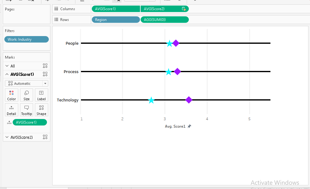
Step-9
Please look below image for reference.

Customize Line and Shape Chart for 2 value in one line.

Step-1 Open Tableau Desktop

Step-2 Connect Data-source Example like – XYZ data source

Step-3 1. Drag “Region” field dimension into Rows shelf
2. write SUM(0) in Rows shelf

Step-4 1. Drag “Score1” filed measure into Columns shelf
2. Drag “Score2“ filed measure into Columns shelf
3. RIght click on “Score2“ and select Dual axis
4. Right Click on Exis value and select Synchronize axis.

Step-5 Go to “Score1” Mark Shelf -> Shape -> Select shape as per your preference.

Step-6 Go to “Score2“ Mark Shelf -> Shape -> Select shape as per your preference.

Step-7 Right click on “SUM(0)“ -> select Formate -> go to Rows Tab -> Zeroline columns u can changes as per your preference.

Please look below image for reference